Large-scale thamamocortical model

While the Blue Brain folk want to construct an incredibly detailed model of a single cortical column, a recent paper by Izhikevich and Edelman (Large-scale model of mammalian thalamocortical systems) reports on a less detailed model of the entire human thalamocortical system.

Some of the details of their model (roughly from large-scale to lower scale) include:
1. The cortical sheet's geometry was constructed from human MRI data.
2. Projections among cortical regions were modeled using data from diffusion tensor MRI of the human brain (above image is Figure 1 of the paper showing a subset of such connections).
3. Synaptic connectivity patterns among neurons within and between cortical layers are based on detailed studies of cat visual cortex (and iterated to all of cortex).
4. Individual neurons are not modelled using the relatively computationally intensive Hodgkin-Huxely models, but a species of integrate-and-fire neuron that included a variable threshold, short-term synaptic plasticity, and long term spike-timing dependent plasticity.
5. The only subcortical structure included in the model is the thalamus, but the model does include simple simulated neuromodulatory influences (dopamine, acetylcholine).

Their model exhibited some very interesting behavior. First, larger-scale oscillatory activity that we see in real brains emerged in the model (e.g., as you would observe via EEG). Also like real brains, the model exhibited ongoing spontaneous activity in the absence of inputs (note this only occurred after an initial 'setup' period in which they simulated random synaptic release events: the learning rule seemed to take care of the rest and push the brain into a regime in which it would exhibit spontaneous activity). Quite surprisingly, they also found that when a single spike was removed from a single neuron, the state of the entire brain would diverge compared to when that spike was kept in the model. There is a lot more, so if this sounds interesting check out the paper. They also mention in the paper that they are currently examining how things change when they add sensory inputs to the model.

Of course, a great deal of work is yet to be done, a great deal of thinking through the implications (and biological relevance) of some of the model's behavior (especially its global sensitivity to single spikes, which to me sounds biologically dubious). However, I find it quite amazing that by simply stamping the basic cortical template onto a model of the entire cortical sheet, and adding the rough inter-area connections, they observed many of the qualitative features of actual cortical activity. We tend to focus so much on local synaptic connections in our models of cortex, it is easy to miss the fact that the long-range projections could have similarly drastic influences on the global behavior of the system.

This paper is just fun. First, it is a great example of how to write a modeling paper for nonmathematicians. It had enough detail to give the modeler a sense for what they did, but not so much detail that your average systems neuroscientist would instinctively throw it in the trash (as is the case with too many modelling papers). Second, it provides a beautiful example of how people interested in systems-level phenomena can build biology into their model without making the model so computationally expensive that it would take fifty years to simulate ten milliseconds of cortical activity. It will be very interesting in the future as the hyper-realist Blue Brain style models make contact with these middle-level theories. I don't see conflict, but a future of productive theory co-evolution.

Visualizing the SVD

Warning: this post isn't directly about neuroscience, but a mathematical tool that is used quite a bit by researchers. 

One of the most important operations in linear algebra is the singular value decomposition (SVD) of a matrix. Gilbert Strang calls the SVD the climax of his linear algebra course, while Andy Long says, "If you understand SVD, you understand linear algebra!" Indeed, it ties about a dozen central concepts from linear algebra into one elegant theorem.

The SVD has many applications, but the point of this message is to examine the SVD itself, to massage intuitions about what is going on mathematically. To help me build intuitions, I wrote a Matlab function to visualize what is happening in each step of the decomposition (svd_visualize.m, which you can click to download). I have found it quite helpful to play around with the function. It takes in two arguments: a 3x3 matrix (A) and a 3xN 'data' matrix in which each of the N columns is a 'data' point in 3-D space. The function returns the three matrices in the SVD of A, but more importantly it generates four plots to visualize what each factor in the SVD is doing.

To refresh your memory, the SVD of an mxn matrix A is a factorization of A into three matrices, U, S, and V' such that:

A=USV'

where V' means the transpose of V. Generally, A is an mxn matrix, U is mxm, S is mxn, and V' is nxn.

One cool thing about the SVD is that it breaks up the multiplication of a matrix A and a vector x into three simpler matrix transformations which can be easily visualized. To help with this visualization, the function svd_visualize generates four graphs: the first figure plots the original data and the next three plots show how those data are transformed via sequential multiplication by each of the matrices in the SVD.

In what follows, I explore the four plots using a simple example. The matrix A is a 3x3 rank 2 matrix, and the data is a 'cylinder' of points (a small stack of unit circles each in the X-Y plane at different heights). The first plot of svd_visualize simply shows this data in three-space:



In the above figure, the black lines are the standard basis vectors in which the cylinder is initially represented. The green and red lines are the columns of V, which form an orthogonal basis for the same space (more about this anon).

When the first matrix in the SVD (V') is applied to the data, this serves to rotate the data in three-space so that the data is represented relative to the V-basis. Spelling this out a bit, the columns of V form an orthogonal basis for three-space. Multiplying a vector by V' changes the coordinate system in which that vector is represented. The original data is represented in the standard basis, multiplication by V' produces that same vector represented in the V-basis. For example, if we multiply V1 (the first column of V) by V, this rotates V1 so that V1 is represented as the point [1 0 0]' relative to the V-basis. Application of this rotation matrix V' to the above data cylinder yields the following:


As promised, the data is the exact same as in Figure 1, but our cylinder has been rotated in three-space so that the V-basis vectors lie along the main axes of the plot. The two green vectors are the first two columns of V, which now lie along the two horizontal axes in the figure (for aficianados, they span the row space of A, or the set of all linear combinations of the rows of A). The red vertical line is the third column of V (its span is the null space of A, where the null space of A is the set of all vectors x such that Ax=0). So we see that the V' matrix rotates the data into a coordinate system in which the null space and row space of A can be more readily visualized.

The second step in the SVD is to multiply our rotated data by the 'singular matrix' S, which is mxn (in this case 3x3). S is a "diagonal" matrix that contains nonnegative 'singular values' of A sorted in descending order (technically, the singular values are the square roots of the eigenvalues of A'*A that correspond to its eigenvectors, which are the columns of V). In this case, the singular values are 3 and 1, while the third diagonal elment in S is zero.

What does this mean? Generally, multiplying a vector x=(x1,....xn)' by a diagonal matrix with r nonzero elements on the diagonal s1,....sr simply yields b=(s1*x1, s2*x2, .... sr*xr, 0 .. 0). That is, it stretches or contracts the components of x by the magnitude of the the singular values and zeroes out those elements of x that correspond to the zeros on the diagonal. Note that S*V1 (where V1 is the first column of V) would yield b=(s1, 0 0 0 0 0). That is, it yields a vector whose first entry is s1 and the rest zero. Recall this is because S acts on vectors represented in the V-basis, and in the V-basis, V1 is simply (1,0, ..., 0).

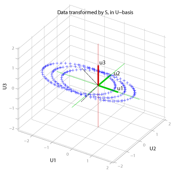
Application of our singular matrix to the above data yields the following:



This 3-D space represents the outputs space (range) of the A transformation. In this case, the range happens to be three-space, but if A had been Tx3, the input data in three-space would be sent to a point in a T-dimensional space. The figure shows the columns of the matrix U (in green and red) are aligned with the main axes: so the transform S returns values that are in the range of A, but represented in the orthogonal basis set in U. The green basis vectors are the first two columns of U (and they span the column space of A), while the red vector is the third column of U (which spans the null space of A').

Since the column space of A (for this example) is two dimensional, any point in 3-D space in the input space (the original data) is constrained to be projected onto a plane in the output space.

Notice that the individual circles that made up the cylinder have all turned into ellipses in the column space of A. This is due to the disproportionate stretching action of the singular values: the stretching is maximum for the vectors in the direction of V1. Also note that in the U-basis, S*V1 lies on the same axis as U1 (U1, in the U-basis, is of course (1, 0, 0)), but s1 units along that axis for reasons discussed in the text after Figure 2.

One way to look at S is that it implements the same linear transformation as the matrix A, but with the inputs and outputs represented in different basis sets. The inputs to S are the data represented in the V-basis, while the outputs from S are the data represented in the U-basis. That makes it clear why we first multiply the data by V': this changes the basis of the input space to that which is appropriate for S. As you might guess, the final matrix, U, simply transforms the output of the S transform from a representation in the U-basis back into the standard basis.

Hence, we shouldn't be surprised that the final step in the SVD is to apply the mxm (in this case, 3x3) matrix U to the transformed data represented in the U-basis. Just like V', U is a rotation matrix: it transforms the data from the U-basis (above picture) back to the standard basis. The standard basis vectors are in black in the above picture, and we can see that the U transformation brings them back into alignment with the main axes of the plot:



Pretty cool. The SVD lets you see, fairly transparently, the underlying transformations implicitly lurking in any matrix. Unlike many other decompositions (such as a diagonalization), it doesn't require A to have any special properties (e.g., A doesn't have to be square, symmetric, have linearly independent columns, etc). Any matrix can be decomposed into a change of basis (rotation by V'), a simple scaling (and "flattening") operation (by the singular matrix S), and a final change of basis (rotation by U).

Postscript: I realize this article uses a bit of technical jargon, so I will post a linear algebra primer someday that explains the terminology. For the aficianados, I have left out some details that would have complicated things and made this post too long. In particular, I focused on how the SVD factors act on "data" vectors, but little on the properties of the SVD itself (e.g., how to compute U, S, and V; comparison to orthogonal diagonalization, and tons of other things).

If you have suggestions for improving svd_visualize, please let me know in the comments or email me (thomson ~at~ neuro [dot] duke -dot- edu).

Edit in 2022: it has been almost 15 years since I made this post. It has held up fairly well as one Gilbert-Strang-like take on SVD, but I wrote it as if V and U are always rotation matrices when you perform SVD. This is not right: they can be either rotation or reflection matrices (the latter have a determinant of -1, while the former have a determinant of 1). For the example used in the code here, the determinants are 1 so we have rotation matrices, but this will not always be the case. Note a reflection is when certain axes flip (e.g., like going from a right to a left-handed coordinate system), so is similar to a rotation, but is mathematically not the same.